Comparing Markov Chain Monte Carlo and Variational Methods for Bayesian Inference on Mixtures of Gamma Distributions

My 2019 honours thesis on variational inference for finite mixtures of gamma distributions.

This was my 2019 honours thesis at the University of Western Australia, supervised by John Lau and Edward Cripps. I studied finite mixtures of gamma distributions and compared a Gibbs sampler with two coordinate-ascent variational methods.

A large part of the work was deriving usable variational updates. One awkward term is

\mathbb{E}_{q(\alpha_k)}\!\left[\log \Gamma(\alpha_k)\right],

which has no convenient closed form. I approximated it with Taylor expansions around the variational mean, using Stirling approximations where they simplified the resulting expressions.

Shape and mean

The larger improvement came from changing the parameterisation of each gamma component. Gamma distributions are usually written in terms of shape $\alpha$ and rate $\beta$ . Those parameters are strongly coupled in the posterior, which is a poor fit for a mean-field approximation that treats them as independent.

The Fisher information in shape-rate coordinates contains off-diagonal terms:

I(\alpha,\beta) = N \begin{bmatrix} \psi^{(1)}(\alpha) & -1/\beta \\ -1/\beta & \alpha/\beta^2 \end{bmatrix}.

Using the mean $\mu=\alpha/\beta$ instead of the rate diagonalises it:

I(\alpha,\mu) = N \begin{bmatrix} \psi^{(1)}(\alpha)-1/\alpha & 0 \\ 0 & \alpha/\mu^2 \end{bmatrix}.

The thesis calls the original shape-rate approximation VI-1 and the shape-mean version VI-2. VI-2 is fitted in the better coordinate system and transformed back when needed. The difference is visible in the posterior itself.

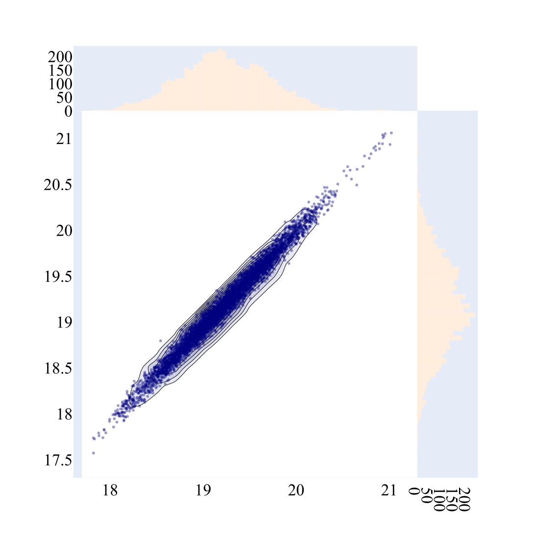
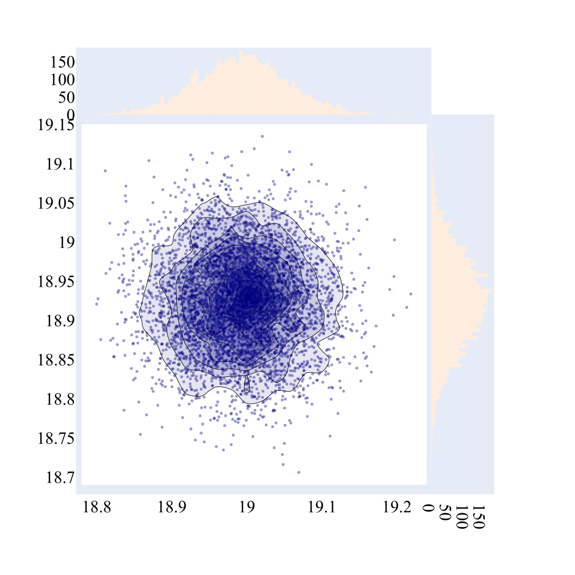
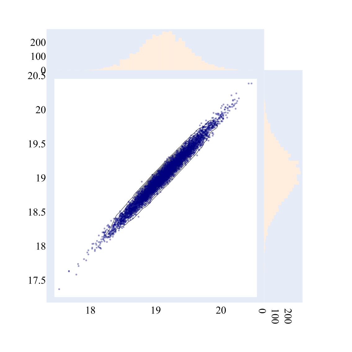
MCMC posterior density in shape-rate coordinates, showing a broad diagonal dependence between the two parameters. — Posterior density for one mixture component in shape-rate coordinates. VI-1 cannot represent the diagonal dependence. VI-2 is fitted in shape-mean coordinates and recovers most of it when transformed back.

VI-1 posterior density in shape-rate coordinates, collapsed into a much narrower approximation. — Posterior density for one mixture component in shape-rate coordinates. VI-1 cannot represent the diagonal dependence. VI-2 is fitted in shape-mean coordinates and recovers most of it when transformed back.

In the experiments, VI-2 also converged faster than VI-1 and gave much better posterior variance estimates at essentially the same computational cost.

Implementation and results

MixGammaVI is the TensorFlow 2 and TensorFlow Probability implementation I wrote for the thesis. The public API was small:

params = mix_gamma_vi(x, K=5)

On one synthetic timing experiment, VI-2 fitted a 14-component model in 0.493 seconds. The Gibbs implementation took 31.380 seconds. These are timings for the implementations and stopping rules used in the thesis, not a general comparison between MCMC and variational inference.

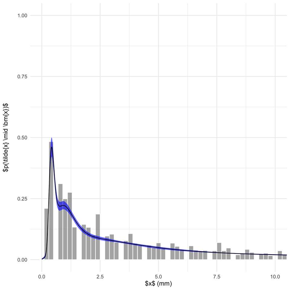
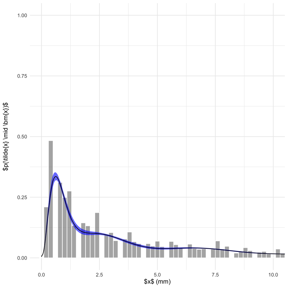
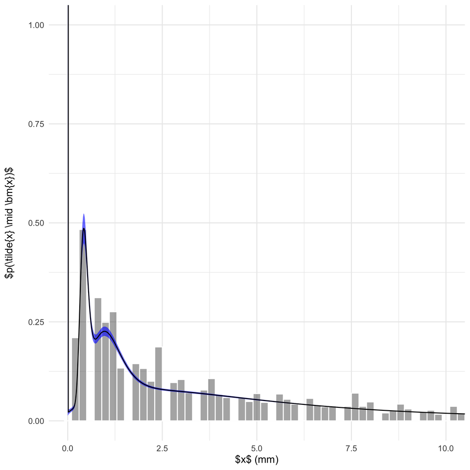
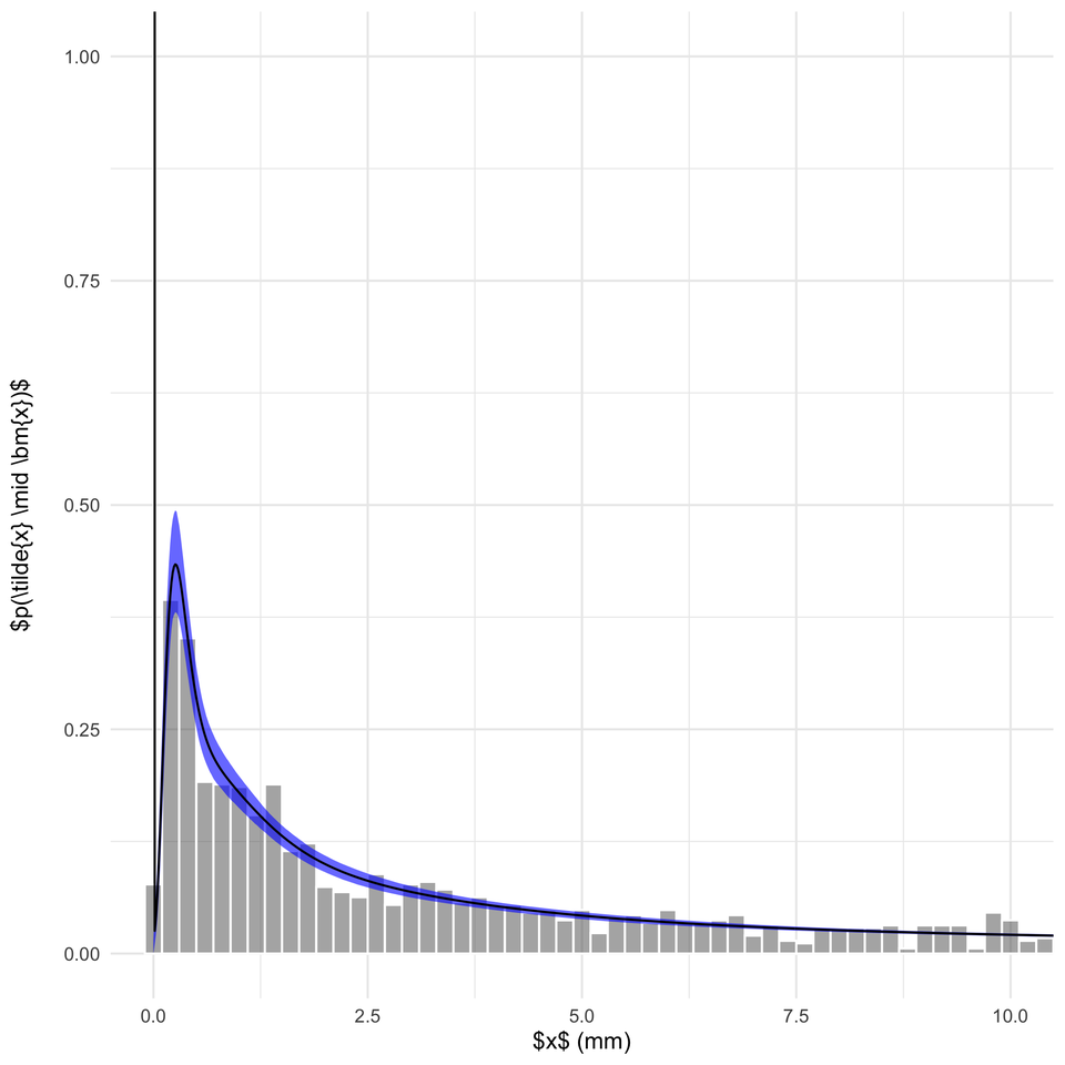
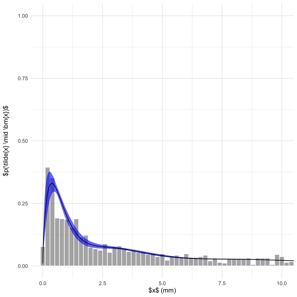
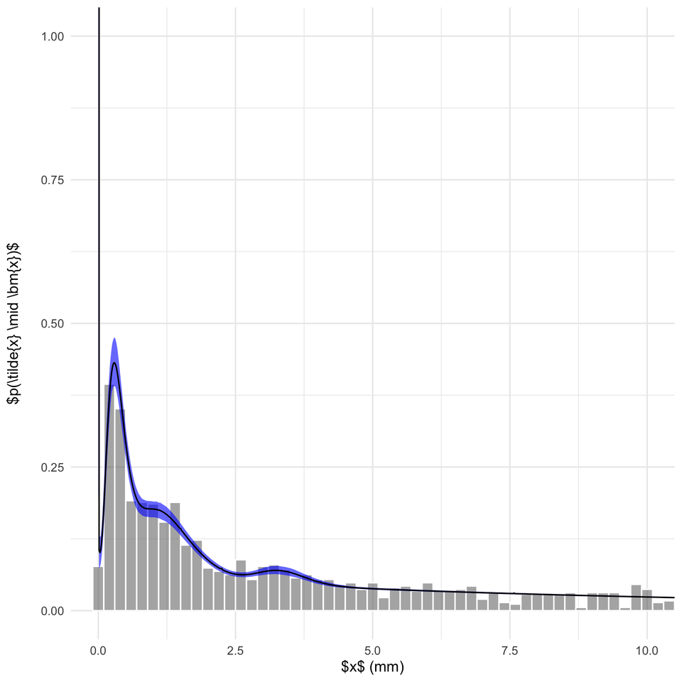
The applied experiment used daily rainfall from four Australian dams. The Woronora and Wellington results below are the most useful pair to keep here. All three methods capture the main mass of the distribution; at Wellington, VI-2 also finds smaller modes that the other two fits miss.

MCMC posterior predictive density and interval for daily rainfall at Woronora Dam. — Posterior predictive densities and 90% intervals for Woronora and Wellington. VI-2 resolves three modes at Wellington in this fit.

VI-1 posterior predictive density and interval for daily rainfall at Woronora Dam. — Posterior predictive densities and 90% intervals for Woronora and Wellington. VI-2 resolves three modes at Wellington in this fit.

Read the thesis

Open the PDF directly if the embedded reader is unavailable.

There are limits worth keeping with the result. The Gibbs implementation had an initialisation bug above fourteen components, mean-field inference still tends to underestimate posterior variance, and the rainfall model omitted zero-rainfall days and temporal dependence.

The full thesis contains the derivations, experiments and extensions in detail.